Market Cycle Prediction Model - Data Analysis
published October 31, 2020
Introduction
This article is the second part of a three-part series of articles with the overriding goal of developing an ML model for predicting market cycles. The model is useful on its own as a buy/sell signal, as input to broader investment strategy, or for use as an input to another model. Such a market cycle prediction model is not available to the open-source community. Thus, an additional goal is to publish the model and methods to the open-source software community. Furthermore, the same process used here to model the S&P 500 works for individual securities.
After a brief articulation of the objectives and importing the necessary data, in this article, we thoroughly analyze the data needed to create the predictive model. Data analysis is a crucially important exercise for developing an effective ML model. The model development process’s data analysis phase requires an organized and systematic approach. Data analysis can be a tiring effort, and data scientists can feel rushed to get to the modeling phase. However, very often, data understanding and data processing is the key to building an accurate model. A thorough understanding of the data and its relationship to the business often yields significant and valuable insights.
This article implements the first three phases of the data science modeling process. Thus, as we proceed, it will be helpful to keep in mind this process and the relationship to our exercise. The first three steps of the process are listed below.
- Objective: The first step in the process is to layout the business and technical objectives. We describe the goals for this ML exercise below.
- Data Wrangling - This stage requires acquiring the data, data manipulation, data modeling (e.g., schema design) in preparation for analysis. Below, this step is discussed in the “Data Import” and “Data Transform” sections. Data sources useful for stock market prediction are daily market performance and economic variables such as consumer sentiment, unemployment rate, long-term, short-term bond rates, market price/earnings ratio, GDP, and market cycle information (form Part 1).
- EDA (Exploratory Data Analysis) - In the EDA stage, we explore the data, extract features useful for Machine Learning, and develop a hypothesis for the type of ML or AI model to solve the problem. In this article, the EDA process is performed in the “Data Transforms” and “Data Analysis Sections.”
Outline
- Objectives
- Github Links
- Notebook Initialization
- Data Import
- Data Transformations and Joins
- Data Analysis
- Correlations
- Save the ML dataframe
- Summary and Conclusions
- References
Objectives
The first step in the data science modeling process is to understand the business and technical objectives. In this case, the aim is to predict market down and upcycles to guide investments, buy and sell, in the stock market. In this case, the objective is to predict the mkt (dependent variable), which indicates a “Bull” up-trending market, or “Bear” down-trending market. The mkt variable was derived from the S&P 500 close price in the previous article (part 1.) This objective, buy or sell signal, will, in turn impose technical requirements on the prediction model. To be practically useful, the predicted investment signal (prediction of mkt) will need to be highly accurate, including high precision and selectivity. Investors are not likely to base investment decisions on a signal that is not highly accurate. False positives, falsely predicting a downward trending (Bear), will cause de-investment of potentially large investments, incur fees, and miss out on upward trends, resulting in losses. Similarly, false negatives will keep money invested in a downward trending market and incur a financial loss. Generally, a low performing signal will not garner the confidence necessary for adoption by market professionals.
An additional requirement for this project is the use of open-source data. Market analysts often have access to superior data sources that provide valuable and insightful data. These special data sources are often available to financial investment institutions at a significant cost. However, this exercise is an open-source project and will demonstrate that creating an accurate model with open data sources is possible. The data and software for creating an accurate market cycle model are made available to the open-source community in the Pyqunt python module available in Github.
Github Links
The software for this post is contained in the Pyquant GitHub repository. Specifically, the following modules and notebooks from the repository are used to support the analysis and results for this post.
- fmplot - plot financial time-series data including sub-plots, line plots, and market cycle (stem) plots.
- fmget - get and manage financial and economic data from various APIs
- fmtransforms - transformations to support market financial analytics
- fmcycle - derive financial market cycles up and down trends (“Bull”, “Bear”) from stock data
- Initial Data for Each Data Source
- “SP500_MktCycle_Data_2” - Notebook with code for this article.
Notebook Initialization
import pandas as pd
import numpy as np
import matplotlib.pyplot as plt
import datetime as dt
from datetime import timedelta as td
import seaborn as sns
import quandl

%run fmget
%run fmtransforms
%run fmplot
%run fmcycle
The python code for the examples discussed in this article is contained in the “SP500_MktCycle_Data” notebook (link above).
We begin by importing packages and modules. The fmget.py, fmtransforms.py, fmcycle.py, and fmplot.py are not available within a python package. Thus, using the software requires downloading into a directory contained in the PYTHONPATH. Downloading the modules into the Jupyter or Python working directory is typically the most straightforward approach.
Data important
The data import examples herein demonstrate how to import data from public APIs using functions within the fmget.py module and transform the data for subsequent analysis with functions from the fmtransforms.py module.
Importing Raw Data from APIs
The code block below first imports data from the existing set of saved data files. If the parameter update_data is equal to True, then the current data is augmented with new information acquired from several publicly available APIs. Setting the start and end datetime variables indicates to get data only over the corresponding dates. fmget.py facilitates a simple data management level by appending new data to the existing data sources and saving the updated data into the specified directory. The files’ names are updated automatically based on the acquired data, start, and end dates in the corresponding dataframe. This process enables archiving data for when recovery is needed or the API sources are unavailable.
To get started, when existing data is not yet available, new data can be downloaded manually from the corresponding sources. Or, an initial set of data for each of these sources is available in Github.
The data import is facilitated by several functions within the fmget.py module, as follows.
- Yahoo - yahoo_getappend() acquires data from a specific symbol from Yahoo Finance and appends it to the existing data.
- Quandl - quandl_sppe_getappend() acquires price to earnings data from the Quandle API. A Quandle API Key will be required. The API key is loaded from a file in the current working directory (see code below).
- FRED - fred_getappend() acquires data (“series”) from the FRED (St. Louis Federal Reserve Bank of St. Louis). This API also requires an API key. Similarly, the API key is loaded from a file in the current working directory (see code below).
The following data are acquired from open APIs.
- S&P 500 daily stock prices, acquired from S&P500 Yahoo, updated daily.
- S&P 500 Price/Earnings is acquired from Quandl. The P/E ratio is reported monthly. Fmget then extrapolates an earnings number (for the past year) from the trailing year P/E, and then the daily P/E is computed using the S&P 500 close price.
- T10Y3M - The spread between 10-year treasury yield to 3-month treasury yield, reported daily, acquired from the FRED API.
- GDP - Gross Domestic Product, reported quarterly and acquired from the FRED API.
- UNRATE - Unemployment Rate reported monthly, acquired from the FRED API.
- CPIAUCSL - Consumer Price Index (CPI), reported monthly and acquired from the FRED API.
- UMCSENT - University of Michigan consumer sentiment, reported monthly, acquired from the FRED API.
On some occasions, data may be reported less frequently than indicated above due to extenuating circumstances, for example, as during the COVID-19 pandemic. Such situations have occurred for the acquisition of P/E and Consumer Sentiment. In such cases, we proceed by filling forward until new data is available.
Examples (a couple of rows) for each of the corresponding dataframes are shown below the code block.
# get recessions
recessions = get_recessions()

# Data files with current set of data

sp500_file = './data/GSPC_1950-1-3_to_2020-10-5.csv'
sppe_file='./data/sp500_pe_daily_1950-1-3_to_2020-10-5.csv'
t10y3m_file='./data/T10Y3M_1982-1-4_to_2020-10-5.csv'
gdp_file='./data/GDP_1947-1-1_to_2020-4-1.csv'
unrate_file='./data/UNRATE_1948-1-1_to_2020-9-1.csv'
cpiaucsl_file='./data/CPIAUCSL_1947-1-1_to_2020-8-1.csv'
umcsent_file='./data/UMCSENT_1953-2-1_to_2020-8-1.csv'


# read in Files with the current set of data
df_sp500 = pd.read_csv(sp500_file,index_col=0,parse_dates=True)
df_sppe_daily = pd.read_csv(sppe_file,index_col=0,parse_dates=True)
df_t10y3m =pd.read_csv(t10y3m_file,index_col=0,parse_dates=True)
df_gdp = pd.read_csv(gdp_file,index_col=0,header=0,parse_dates=True)
df_unrate = pd.read_csv(unrate_file,index_col=0,header=0,parse_dates=True)
df_cpiaucsl = pd.read_csv(cpiaucsl_file,index_col=0,header=0,parse_dates=True)
df_umcsent = pd.read_csv(umcsent_file,index_col=0,header=0,parse_dates=True)

# update data and append, if update_data == True
update_data=False

if update_data==True:
    print('today =',dt.datetime.today())
    start=dt.datetime(2020,8,1)  # update data start
    end=dt.datetime(2020,10,6)   # update data end

    # Quandle API key
    quandle_api_key_file = "quandl_api_key_file"
    f = open(quandle_api_key_file,'r')
    quandl_api_key=f.read().strip()
    f.close

    # Fred API key
    fred_api_key_file = "fred_api_key_file"
    f = open(fred_api_key_file,'r')
    fred_api_key=f.read().strip()
    f.close

    df_sp500=yahoo_getappend('^GSPC',start,end,df=df_sp500,save=True,savedir='./data')
    df_sppe_daily=quandl_sppe_getappend(df_sppe_daily,df_sp500,quandl_api_key, start,end,save=True, savedir='./data')
    df_t10y3m=fred_getappend('T10Y3M',start,end,df=df_t10y3m,API_KEY_FRED=fred_api_key,save=True,savedir='./data')
    df_gdp=fred_getappend('GDP',start,end,df=df_gdp,API_KEY_FRED=fred_api_key,save=True,savedir='./data')
    df_unrate=fred_getappend('UNRATE',start,end,df=df_unrate,API_KEY_FRED=fred_api_key,save=True,savedir='./data')
    df_cpiaucsl=fred_getappend('CPIAUCSL',start,end,df=df_cpiaucsl,API_KEY_FRED=fred_api_key,save=True,savedir='./data')
    df_umcsent=fred_getappend('UMCSENT',start,end,df=df_umcsent,API_KEY_FRED=fred_api_key,save=True,savedir='./data')


    display(df_sp500.tail(2))
    display(df_t10y3m.tail(2))
    display(df_sppe_daily.tail(2))
    display(df_gdp.tail(2))
    display(df_unrate.tail(2))
    display(df_cpiaucsl.tail(2))
    display(df_umcsent.tail(2))
              Close      	High	    Low	   Open	   Volume	   Adj Close
Date
2020-10-02  	3348.419	3369.100	3323.690	3338.939	3.961e+09	3348.419
2020-10-05  	3408.600	3409.570	3367.270	3367.270	3.686e+09	3408.600

T10Y3M
index
2020-10-02	0.61
2020-10-05	0.68

            PE	Earnings
Date
2020-10-02	28.781	116.339
2020-10-05	29.299	116.339

            GDP
index
2020-01-01	21561.139
2020-04-01	19408.759

            UNRATE
index
2020-08-01	8.4
2020-09-01	7.9

            CPIAUCSL
index
2020-07-01	258.723
2020-08-01	259.681

          UMCSENT
index
2020-03-01	89.1
Market Cycles
In the code block bellow, the market cycles are imported from a file or computed from newly available S&P price data. When the compute variable is set equal to 1, the cycles are derived from S&P close price. When compute = 0, the market cycle information is loaded from a saved file. This latter option is convenient to save time since it takes a few minutes to compute the market cycles for the market history going back to 1950. However, when analyzing the data and restarting the notebook, it is unnecessary to recompute the market cycles when the market data has not changed. The fmcyle() function was discussed in detail in the previous post Analyzing Bull and Bear Market Cycles in python. A couple rows of the detailed market cycle dataframe (dfmc) are listed following the code block.
#Market Cycles

%run fmtransforms
%run fmplot
%run fmcycle
compute=0   # if compute is 1 then compute new market cycles, else load from saved file

f_dfmc="./data/GSPC_dfmc2020.5_1950_2020-10-5.csv"
f_dfmcs="./data/GSPC_dfmcs2020.5_1950_2020-10-5.csv"

mcycledown=20
mcycleup=20.5

#string = get_market_cycles()

df_mc,df_mcsummary=fmcycles(df=df_sp500,symbol='GSPC',compute=compute, mc_filename=f_dfmc, mcs_filename=f_dfmcs, mcdown_p=mcycledown,mcup_p=mcycleup,savedir="./data")

display(df_mc.tail(2))
            Close	    High    	Low	      Open	   Volume  	  Adj Close mkt	mcupm	mcnr	mucdown	mdcup
Date
2020-10-02	3348.420	3369.100	3323.690	3338.940	3.962+09	3348.420	1	1	0.497	0.0650	0.0
2020-10-05	3408.600	3409.570	3367.270	3367.270	3.687e+09	3408.600	1	1	0.523	0.0481	0.0
Data Transformations and Joins
Now that we have the necessary data, we need to apply several transformations to make it useful. For reference, we reviewed the data science modeling process in a previous article. In this article, the process of Exploratory Data Analysis (EDA) occurs in this section (“Data Transformations and Joins”) and the next section (“Data Analysis”).
The transformations and joins will generate one dataframe, df_ml, with all the machine learning features. It is essential to keep in mind that the feature extraction exercise will create the ML features, where the main focus is creating variables that appear useful for ML. However, potentially more variables than necessary may result. In the feature selection process, during model development, we will decide to use some, not all, of the features based on their usefulness to the predictive model.
df_ml=pd.DataFrame()

# Join PE, Earnings and Market Cycles
# Drop Adj Close, does not make sense for S&P
# Compute Earnings percent return
df_sppe=period_percent_change(df_sppe,'Earnings',new_variable_name = 'Earnings_mom')
df_sppe=period_percent_change(df_sppe,'PE',new_variable_name = 'PE_mom')
df_ml=fmjoinff(df_mc,df_sppe[['PE','PE_mom','Earnings','Earnings_mom']],verbose=False,dropnas=True).drop(['Adj Close'],axis=1)


# Yield Curve, T10Y3M, 10 Year Treasury - 3 Month Treasury
df_ml=fmjoinff(df_ml,df_t10y3m,verbose=False,dropnas=True)

# GDP
df_gdp = gdprecession(df_gdp,'GDP') # adds gdg_qoq, recession1q, recession2q
df_ml=fmjoinff(df_ml,df_gdp,verbose=False,dropnas=True)

# Unemployment
df_unrate=period_percent_change(df_unrate,'UNRATE',new_variable_name='unrate_pchange')
df_ml=fmjoinff(df_ml,df_unrate,verbose=False,dropnas=True)

# Consumer price index
df_cpi=period_percent_change(df_cpiaucsl,'CPIAUCSL',new_variable_name='cpimom')
df_ml=fmjoinff(df_ml,df_cpi[['CPIAUCSL','cpimom']],verbose=False,dropnas=True)

# Consumter Sentiment
df_umcsent=period_percent_change(df_umcsent,'UMCSENT',new_variable_name='umcsent_pchange')
df_ml=fmjoinff(df_ml,df_umcsent,verbose=False,dropnas=True)


# Simple Moving Averages
df_ml=dfsma(df_ml,'Close',windows=[20,50,200])

# Normalized mavgs
#   1-day (today / yesterday .... sma5 = 5-day smavg( today / yesterday ) .... )
df_ml=dfnma(df_ml,['Close','Volume'],windows=[1,5,10,15,20,30,50,200])

# Relative 200-day moving average
# scale of 0 to 1
df_ml=dfrma(df_ml,'Close_sma50','Close_sma200',varname='rma_sma50_sma200')
df_ml=dfrma(df_ml,'Close_sma20','Close_sma50',varname='rma_sma20_sma50')

# ADX
df_ml=dfadx(df_ml,'Close','High','Low',window=50)

# Volatility ... Log Return Std Dev, and Velocity
df_ml=dflogretstd(df_ml,'Close',windows=[25,63,126])
df_ml=dfvelocity(df_ml,'Close_lrstd25',windows=[5])
df_ml=dfvelocity(df_ml,'Close_lrstd63',windows=[5])
df_ml=dfvelocity(df_ml,'Close_lrstd126',windows=[5])

print(df_ml.columns)
Index(['Close', 'High', 'Low', 'Open', 'Volume', 'mkt', 'mcupm', 'mcnr',
 'mucdown', 'mdcup', 'PE', 'Earnings', 'T10Y3M', 'GDP', 'gdp_qoq',
 'recession1q', 'recession2q', 'UNRATE', 'UNRATE_avgvel3', 'CPIAUCSL',
 'cpimom', 'UMCSENT', 'UMCSENT_avgvel3', 'Close_sma20', 'Close_sma50',
 'Close_sma200', 'Close_nma1', 'Volume_nma1', 'Close_nma5',
 'Volume_nma5', 'Close_nma10', 'Volume_nma10', 'Close_nma15',
 'Volume_nma15', 'Close_nma20', 'Volume_nma20', 'Close_nma30',
 'Volume_nma30', 'Close_nma50', 'Volume_nma50', 'Close_nma200',
 'Volume_nma200', 'rma_sma50_sma200', 'rma_sma20_sma50', 'PDI50',
 'NDI50', 'ADX', 'Close_lrstd25', 'Close_lrstd63', 'Close_lrstd126',
 'Close_lrstd25_avgvel5', 'Close_lrstd63_avgvel5',
 'Close_lrstd126_avgvel5'],
dtype='object')
The transformations and joins are performed in the code block (above) are briefly described below. Each of the transformations is supported by functions contained in the fmtransforms.py module.
- The fmjoinff() function joins the detailed market cycle dataframe df_mc, and SP 500 price-earnings dataframe. The fmjoinff() function will fill forward and drop NA columns corresponding to any non-market days. We also generate and include the PE month over month and earnings month over month variables. However, in this specific case, the df_ml and df_spee_daily there no NAs and, therefore, no drops.
- The gdprecession() function calculates the quarterly percent change gdp_qoq (GDP this quarter / GDP last quarter - 1) and adds it to the df_gdp dataframe. These variables are joined to the df_ml dataframe with fmjoinff(). In this case, there is only one GDP reported per quarter. The fill forward functionality will fill the missing values so that there are valid GDP numbers for each day, corresponding to the previously reported GDP.
- Similarly, month over month consumer price index is calculated by the cpimom() function and joined into the df_ml data frame with fill forward to fill in missing values.
- The consumer sentiment month over month change is calculated by the period_percent_change() function. As will be observed during the analysis phase below, we will see that the CPIAUCSL direction (positive or negative) is correlated with market cycles. The consumer sentiment (CPIAUCSL) is then joined into the df_ml data frame, and the monthly values are filled forward.
- Momentum variables are calculated with simple moving averages, dfsma() function, of the close price. These variables are not detrended as is required in machine learning but are useful later for human interpretation.
- For machine-learning purposes, normalized moving averages are computed by averaging the normalized 1-day price difference (close price today / close price yesterday - 1). As shown in the code block, the moving averages are computed over the windows of [1,5,10,15,20,30,50,200]. The resulting variables are added to the df_ml data frame by the dfnma() function.
- Often, investors use the relative difference between the 50-day and 200-day moving averages as trading signals. The 50-day moving average crossing above the 200-day moving average is interpreted as a buy, and 50-day crossing below the 200-day moving average is interpreted as a sell signal. The dfrma() function takes a ratio of the input variables and returns them as columns in the df_ml dataframe. The relative 50-day and 200-day movements are computed for close price and volume.
- The Average Direction Index (ADX) is used to determine if the price is trending strongly in the positive or negative direction.$^{2}$ The dfadx() function computes the ADX with the indicated window averaging period as input (50-days as shown below).
- Volatility measures indicate market stability. The standard financial method to measure volatility is with log return standard deviation.$^{2}$ The dflogretstd() function computes the log return standard deviation over indicated averaging windows, 25, 63, 126, as shown below. Finally, the complete list of variables included in the df_ml dataframe is listed below the code block.
Data Analysis
Though there are numerous data from various sources, it will help to organize our analysis into a few salient categories, as follows.
- Economic Indicators - Indicators such as gross domestic product, consumer sentiment, yield curve, and employment that impact the market performance
- Price/Earnings - The market PE ratio represents the forward-looking price valuation to trailing earnings.
- Market Momentum - Market trend indicators include moving averages and average directional index.
- Volatility - Volatility is a measure of market stability.
Economic Indicators
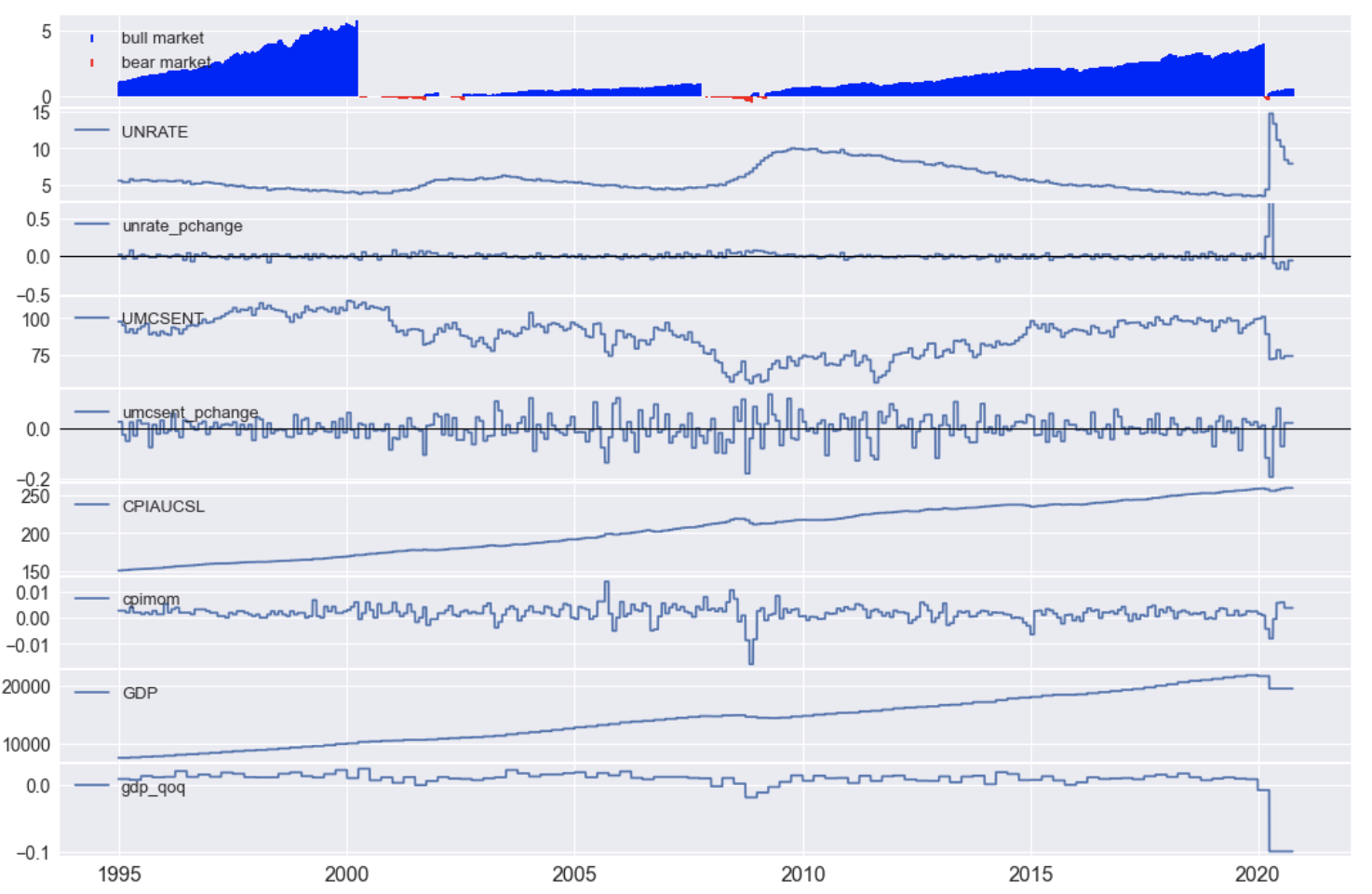
We previously imported several economic indicators, and these, along with data transformations are illustrated in Figure 1. It is useful to Zoom into a period, including a few market cycles, and observe the market behavior relative to the economic indicators.
- The unemployment rate (UNRATE), illustrates correlation to the market up and down cycle. As noted in Part 1, the unemployment rate is a lagging indicator. UNRATE falls and seems to reach a low point before a market crash, as the market hits its peak. On the other hand, unemployment tends to rise when the market hits a low point. We capture the unemployment rate’s direction in the variable unrate_pchange (“Unemployment Percent Change”).
- Consumer sentiment (UMCSENT) falls during down cycles and often at the peak of the market is running at close to 100%. As with the unemployment rate, the directional change in the unemployment rate is significant. Consumer sentiment falls during a market down cycle and rises as the market comes out of a down period.
- The consumer price index (CPI) variable (CPIAUCSL) shows a long term rising trend and will need to be detrended to be useful as an ML feature. To this end, the cpimom variable contains the percent change from one month to the next.
- Like the CPI, the GDP requires detrending, and therein the gdp_qoq variable contains a quarter on quarter percent change.
s=dt.datetime(1995,1,1)
e=dt.datetime(2020,10,5)

fmplot(df_ml,variables=['mcnr','PE','PE_mom','Earnings','Earnings_mom'],plottypes=['mktcycle','line','line','line','line'],
       sharex=True, hspace=0.03, startdate=s,enddate=e, figsize=[18,10],
       xtick_labelsize=16, ytick_labelsize=14,legend_fontsize=13 )
Price Earnings
The price to earnings ratio, PE variable, is a ratio that measures the current market price relative to trailing earnings. The S&P 500 historical average P/E ratio, going back to 1971, is 19.4. For various reasons, the ratio will deviate from this average. Herein we make several observations that will help towards deriving ML features.
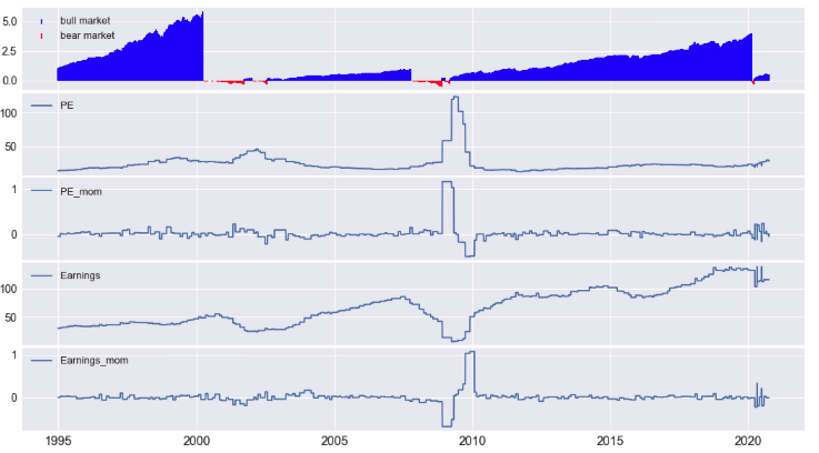
- The PE ratio is based on price from forward-looking expectations and can turn inordinately positive during the initial part of an up cycle. Earnings typically fall when the economy slows down, and thus prices based on future valuations can lead to an inordinately high P/E ratio, especially when the trailing earnings have fallen and forward expectations are high. Though awkward from a financial perspective, this situation can serve as useful predictive input to the ML model. For example, in Figure 2, as expected, we see earnings fall during market down cycles, and with positive forward looking earnings expectations prices will be high leading to an inordinately high P/E ratio.
- The relationship to a market change (e.g., up to down cycle) the logic between Price and Earnings seems a bit complex. In the crash of 2000 Earnings are rising, while overall P/E is falling. In 2007, P/E appears to rise while trailing earnings are falling. In 2020, Earnings are flat, P/E is flat, however MCNR is inflated when the world pandemic strikes.
s=dt.datetime(1995,1,1)
e=dt.datetime(2020,10,5)

fmplot(df_ml,variables=['mcnr','PE','Earnings','Earnings_mom'],plottypes=['mktcycle','line','line','line'],
       sharex=True, hspace=0.03, startdate=s,enddate=e, figsize=[18,6],
       xtick_labelsize=16, ytick_labelsize=14,legend_fontsize=13 )
Momentum - Moving Averages
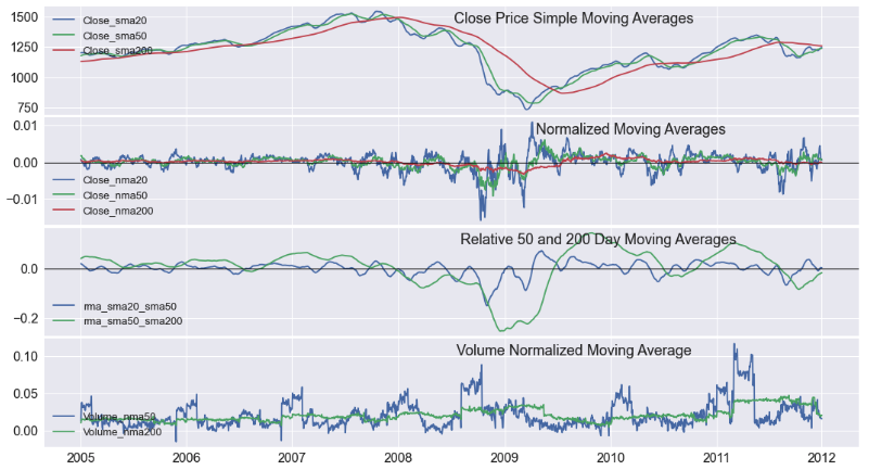
Momentum investing relies on making buy and sell decisions from trends derived in the market moving averages. For example, typical averages for momentum investing are the 50-day and 200-day moving average. A typical technical strategy is to observe when the 50-day moving average crosses above or below the 200-day moving average to make a buy or sell decision, respectively. In our case, first, the variable close_price is de-trended (today’s price / yesterday price - 1) followed by an n-day moving average to generate the variables, such as Close_nma20, Close_nma50, and Close_nma200.
- An example of momentum buy-sell signals is seen in the graph. We see the 50-day moving average cross below the 200-day moving average in late 2008 during the Financial crisis, and then back up as the market turns positive in mid-2009.
- We also see the 50-day volume measure cross above and below the 200-day measure during significant market movements.
startdate = dt.datetime(2005,1,1)
enddate = dt.datetime(2012,1,1)

titles=['Close Price Simple Moving Averages','Normalized Moving Averages','Relative 50 and 200 Day Moving Averages',
        'Volume Normalized Moving Average']
variables=[ ['Close_sma20', 'Close_sma50', 'Close_sma200'], [ 'Close_nma20', 'Close_nma50','Close_nma200'],
           ['rma_sma20_sma50' ,  'rma_sma50_sma200'],
           ['Volume_nma50','Volume_nma200']]

fmplot(df_ml,variables,titles=titles,startdate=startdate,
          enddate=enddate, llocs=['upper left','lower left','lower left','lower left','upper left'],
          title_fontsize=18, titlein=True, hlines=['',0,0,''],titlexy=[(0.65,0.8),(0.72,0.8),(0.68,0.8),(0.65,0.8)],
          hspace=.025, sharex=True, xtick_labelsize=16, ytick_labelsize=16,legend_fontsize=13, figsize=(18,10))
Momentum - ADX Variables
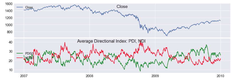
Another set of momentum variables typically employed by investors are the average direction index measures (ADX). Here we have applied a 50-day window to the ADX transforms for generating the variables. We see in Figure 5 the NDI (Negative Direction Index, red) cross above the PDI (Positive Direction Index, green) during downward market movements.
startdate = dt.datetime(2007,1,1)
enddate = dt.datetime(2010,1,1)


titles=['Close', 'Average Directional Index: PDI, NDI']
fmplot(df_ml,['Close',['PDI50','NDI50']],titles=titles,startdate=startdate,
          enddate=enddate,hspace=.03, sharex=True,titlein = True, titlexy=[(0.5,0.83),(0.45,0.85)],
           llocs=['upper left','center left','center left'],
          linecolors=['',['g','r','b']], xtick_labelsize=16, ytick_labelsize=16,
          legend_fontsize=14,title_fontsize=20, figsize=(18,6))
Volatility
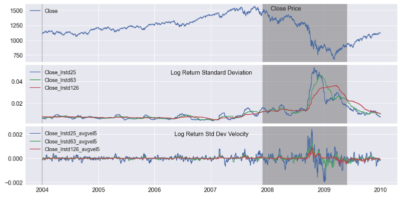
The market volatility is measured with the log return standard deviation and illustrated in Figure 6. During the 2007 - 2009 Financial Crisis, the volatility increases as the market crashes, but volatility falls as the market recovers. As with some of the previous variables, movement velocity (direction) is an important clue. The increasing or decreasing volatility is captured in the “velocity” (difference or derivative) of the log return standard deviation, Close_lrstdxx_avgvel5 variables, and also includes a 5-day running average.
startdate = dt.datetime(2004,1,1)
enddate = dt.datetime(2010,1,1)


fmplot(df_ml,['Close',['Close_lrstd25','Close_lrstd63','Close_lrstd126'],['Close_lrstd25_avgvel5','Close_lrstd63_avgvel5','Close_lrstd126_avgvel5']],
          titles=[ 'Close Price','Log Return Standard Deviation','Log Return Std Dev Velocity'],startdate=startdate,
          enddate=enddate, llocs=['upper left', 'upper left','upper left','upper left'],titlein=True, title_fontsize=16, hspace=0.05,fb=recessions,
          titlexy=[(0.7,0.85),'',''], sharex=True,
          xtick_labelsize=16, ytick_labelsize=16,legend_fontsize=14, figsize=(18,9))
Correlations
Now that we have all our ML features into one dataframe, the next step is to investigate the relationship between the ML features and the target variable and also with other ML Features (multi-collinearity). To do this, we will look at the correlation matrix.
We will also look at how the ML Features are related to a shifted version of the target variable. Because many of the ML features result from sliding window averages, the optimum daily correlation point will be some time in the future. Thus, we will identify the maximum correlation point and use it in the data pre-processing (pre-processing in anticipation of ML) stage to align the features for maximum correlation to the target variable.
Correlation List
We run a pairwise correlation of the variables in the dataframe with the Pandas corr() function. Following the code block, we list the correlations to the target variable, mkt.
We will not comment on every correlation, but we will make a few observations.
- The largest positive correlations are at the top of the list, and largest negative correlations are at the bottom of the list. Variables in the middle of the list are not well correlated to the target.
- Several moving average variables show a strong relationship to the target variable. As expected, the 200-day, 50-day, and 30-day moving averages have a strong relationship with the target variable.
- The MCNR variable, as discussed in Part 1, is not an independent variable and should not be used as a predictor variable.
- Several of the variables generated from fmcycle(), market cycle generation function have good correlation to the target - mcupm, mucdown.
- The volatility variables, log return standard deviation (“lrstd”), show a strong negative correlation.
- The volatility velocity variables (direction of movement) show a good correlation
- Several economic indicators, such as CPIAUCSL (consumer price index), UNRATE (unemployment rate), UMCSENT (consumer sentiment), and the related variables, show a strong correlation.
We have looked at the correlation to the mkt variable one day in advance of the current day. We will see in the next section that we should also consider correlations further out in time. Such a view will cause some variables to have stronger correlations, and thus, they will be more useful as feature variables.
df_ml.drop(['Close_sma20','Close_sma50','Close_sma200'],axis=1,inplace=True)
tmp_remove_cols=['Close','High','Low','Open','Volume','Earnings']
corr_matrix = df_ml.drop(columns=tmp_remove_cols,axis=1).corr()
print(corr_matrix['mkt'].sort_values( ascending = False))
  ['mkt' 'mcupm' 'mcnr' 'mucdown' 'mdcup' 'PE' 'PE_mom' 'Earnings_mom'
   'T10Y3M' 'GDP' 'gdp_qoq' 'recession1q' 'recession2q' 'UNRATE'
   'unrate_pchange' 'CPIAUCSL' 'cpimom' 'UMCSENT' 'umcsent_pchange'
   'Close_nma1' 'Volume_nma1' 'Close_nma5' 'Volume_nma5' 'Close_nma10'
   'Volume_nma10' 'Close_nma15' 'Volume_nma15' 'Close_nma20' 'Volume_nma20'
   'Close_nma30' 'Volume_nma30' 'Close_nma50' 'Volume_nma50' 'Close_nma200'
   'Volume_nma200' 'rma_sma50_sma200' 'rma_sma20_sma50' 'PDI50' 'NDI50'
   'ADX' 'Close_lrstd25' 'Close_lrstd63' 'Close_lrstd126'
   'Close_lrstd25_avgvel5' 'Close_lrstd63_avgvel5' 'Close_lrstd126_avgvel5']
      mkt                       1.000000
      mcnr                      0.407377
      Close_nma200              0.384183
      Close_nma50               0.365427
      Close_nma30               0.336877
      rma_sma50_sma200          0.336456
      rma_sma20_sma50           0.319561
      mcupm                     0.303942
      Close_nma20               0.297762
      Close_nma15               0.272517
      Close_nma10               0.238956
      PDI50                     0.238481
      umcsent_pchange           0.185696
      Close_nma5                0.181201
      UNRATE                    0.139746
      UMCSENT                   0.134231
      GDP                       0.109271
      CPIAUCSL                  0.108861
      Close_nma1                0.087609
      Volume_nma200             0.080180
      T10Y3M                    0.068570
      Earnings_mom              0.067040
      Volume_nma50              0.037872
      Volume_nma30              0.026944
      recession2q               0.025583
      ADX                       0.025054
      Volume_nma20              0.019722
      PE_mom                    0.017526
      Volume_nma15              0.015658
      Volume_nma10              0.009042
      gdp_qoq                   0.007912
      Volume_nma5               0.003342
      Volume_nma1               0.001041
      NDI50                    -0.029316
      PE                       -0.036005
      unrate_pchange           -0.047461
      Close_lrstd25_avgvel5    -0.064506
      recession1q              -0.086878
      mdcup                    -0.089539
      Close_lrstd63_avgvel5    -0.091399
      Close_lrstd126_avgvel5   -0.120839
      Close_lrstd126           -0.130164
      Close_lrstd63            -0.160196
      cpimom                   -0.182724
      Close_lrstd25            -0.196038
      mucdown                  -0.282421
      Name: mkt, dtype: float6
Correlation Heatmap
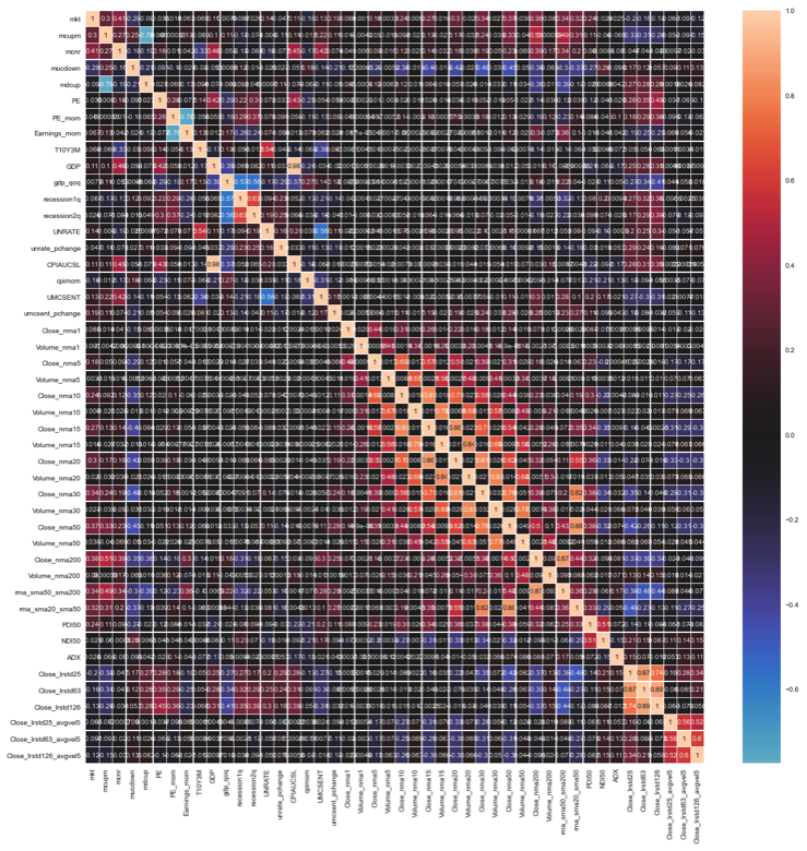
A correlation heatmap is a visual tool for finding strong correlations to the target and pairwise correlated variables. We employ a color scheme where the brightest (lightest color) color represents a high positive correlation, dark (black) represents little or no correlation, and blue represents a strong negative correlation. The bright diagonal is the correlation of each variable to itself. As we did in the previous section, a simple ordered list is the easiest method for finding correlations to the target variable. A heatmap is an excellent tool for identifying the presence of multicollinearity, that is, correlated dependent variables. Such correlations can often work against each other and decrease the predictive performance of the model. Here we see several strongly correlated independent variables. For example, we see a few cross-correlated variables of note.
- Several of the economic indicator variables show cross-correlation.
- The unemployment rate (UNRATE) and the Yield Curve (T10Y3M)
- Gross domestic product (GDP) is strongly correlated to the consumer price index (CPIAUCSL).
- The unemployment rate (UNRATE) has a strong negative correlated to consumer sentiment (UMCSENT)
- Not surprisingly, many of the moving average variables show cross-correlation.
- The market cycle variables also show a strong relationship with several moving averages.
We will deal with the effects of multicollinearity during the feature selection process during the model development phase.
fig, ax = plt.subplots(figsize=(20,20))
sns.heatmap(corr_matrix, center=0, annot=True, linewidths=.3, ax=ax)
plt.show()
Correlation to Shifted Target Variable
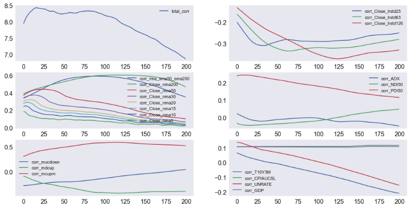
Many of the ML Feature variables are moving averages intended to represent price movements over different periods. Depending on the averaging window, the variable will have an optimal correlation with the target variable sometime in the future. Figure 7 illustrates the correlation with the target variable in the future.
var_list=df_ml.columns
corr_vars = ['corr_'+v for v in var_list]  # name of each = corr_"variable" key for the corr_dict
corr_dict={c : [] for c in corr_vars}     # dictionary of correlations key = "corr_variablename"

total_corr=[]

# iterate over shifted target variable
for k in range(1, 201):
    mkt_n = 'mkt_' + str(k)              # shifted variable name
    df_ml[mkt_n]=df_ml['mkt'].shift(k)   # shifted variable
    corr_matrix = df_ml.corr()           # new correlation matrix
    print(k,end = '.. ')

    # Iterate through dictionary keys and corresponding variables
    for c,v in zip(corr_dict,var_list):
        corr_dict[str(c)].append(corr_matrix[v][mkt_n])  # append correlation to list according to variable key

    df_ml.drop(mkt_n, axis=1, inplace=True)  # drop the shifted target variable

    # add up the total correlations ... approximationdoes not factor in negative cross contributions
    total_corr.append(corr_matrix[mkt_n].abs().sum()-1)


corr_dict.update({'total_corr' : total_corr})
fig,ax = plt.subplots(nrows=3,ncols=2,figsize=[18,9])

corr_list=[
       [['total_corr'] , ['corr_Close_lrstd25','corr_Close_lrstd63','corr_Close_lrstd126']],
       [['corr_rma_sma50_sma200','corr_Close_nma200','corr_Close_nma50','corr_Close_nma30','corr_Close_nma20','corr_Close_nma15','corr_Close_nma10','corr_Close_nma5'], ['corr_ADX','corr_NDI50','corr_PDI50']],
       [['corr_mucdown','corr_mdcup','corr_mcupm'], ['corr_T10Y3M','corr_CPIAUCSL','corr_UNRATE','corr_GDP']],
     ]


for k2 in range(0,3):
    for k1 in range(0,2):
        for key in corr_list[k2][k1]:
            ax[k2,k1].plot(corr_dict[str(key)], label=key)
        ax[k2,k1].legend(loc='upper right')
        ax[k2,k1].grid()
        ax[k2,k1].legend(fontsize=11)
        ax[k2,k1].tick_params( labelsize=16)


plt.show()
The top left curve approximates the total correlation to a future date. Together all the variables show a maximum correlation at about 20 days and a strong correlation to about 100 days.
- On the middle left, we see that the moving averages are maximally correlated to a day approximately 1/2 the window length in the future. For example, the 30 days moving average represents the price movement over 30 days and is maximally correlated to 15 days in the future.
- The relative 200 and 50-day moving averages are maximally correlated to about 100 days in the future.
- The market cycle variables, sown on the bottom left, are strongly correlated one day in the future and show strong correlations to over 100 days. Since the variables are designed to give a short-term warning of a market change, we will employ them unshifted in machine learning.
- The log return standard deviation variables, top right, show a strong correlation to a day in the future a little shorter than the window length.
- The ADX signals, middle right, show their highest correlations at about 25-days out, 1/2 the moving average window length.
- The economic indicators, bottom right, show a strong correlation without a time shift. Some of the variables, such as the Yield curve and Consumer Price index, show a strong correlation over a long period into the future.
These observations will be useful for aligning the independent variables for optimal prediction during the data pre-processing step, where we prepare the ML Features for machine learning.
Save the ML dataframe
Next, we save the final combined data frame of variables so that it can be read into the next phase of processing. Eventually, all the steps in preparing this combined dataframe can be automated and put into an analytics pipeline that feeds the predictive model for a daily market prediction.
today = dt.datetime.today()
startDate=df_ml.index[0]
endDate=df_ml.index[df_ml.index.size-1]
filename='./data/df_ml_'+str(today.year)+str(today.month)+str(today.day)+'_'+str(startDate.year)+str(startDate.month)+\
          str(startDate.day)+'_to_'+str(endDate.year)+str(endDate.month)+str(endDate.day)+'.csv'
print('save filename =',filename)

# save the data index as a column named date
df_ml.reset_index().rename(columns={'index':'Date'}).to_csv(filename,index=False)
Summary and conclusions
This article summarized the first three steps in developing an ML model for predicting S&P 500 market cycles - objectives, data wrangling, and exploratory data analysis. The aim is to provide a buy/sell signal for making investments. The model is also useful as input to other models, and a general indicator of the positive or negative outlook of the stock market.
Several Python modules have been developed to facilitate this process and are available for download on Github. These functions and modules are designed to work together as a system, including fmcycle.py for deriving the market cycles, fmget.py for accessing stock and economic data from public APIs, fmplot.py for easily plotting stock market time-series data, and fmtransforms.py for performing basic transformations needed for EDA on stock data.
The EDA phase of the model development process requires a systematic exploration of the data variables for deriving features useful for machine learning. In this process, we have analyzed several sets of variables, including economic data, momentum variables, and volatility variables. The economic data analyzed include GDP (Gross Domestic Product), CPI (Consumer Price Index), consumer sentiment, and unemployment rate. The data analysis also explored the correlation of the ML features to the target variable and pairwise cross-correlation between them. We packaged all the ML Features into one dataframe, df_ml, for the next step of processing. Automation of this process, creating the df_ml dataframe from raw data, can easily be achieved by packaging all the transformations into an “analytics pipeline” that runs each day.
This article is the second in a three-part series. The first article (Part 1 - Analyzing Bull and Bear Market Cycles in Python) describes how to derive market cycle variables from stock market data. Part 2, this article, covers the first three steps in creating a market cycle prediction model, with emphasis on data analysis and ML feature extraction. The next article, Part 3, begins with the df_ml dataframe created in this article, performs data pre-processing, feature extraction, model training, model testing, and model backtesting.
References
[1] Average Direction Index, Investopedia.
[2] Volatility, Log return standard deviation, Wikipedia.