Time-series Forecasting: from Classical Models to Large-Scale AI Models
published January 15, 2021
last updated January 30, 2021
Introduction
Driven by the digital transformation of business processes, forecasting models are experiencing a significant wave of innovation. Business forecasting as practice goes back thousands of years.$^1$ Today, time-series forecasting models are widely used for business planning across all industry sectors; however, the process is often a small-scale manual exercise. Business forecasting is frequently performed by specialized forecasting experts, human in the loop analysis, and inflexible or hard to tune software models capable of handling single or a few simultaneous (multivariate) time-series. In contrast, modern forecasting model requirements demand - easy to tune models with human interpretable parameters, usability by domain experts (not necessarily forecasting experts), automation without a human in the loop, scalability to thousands or millions of simultaneous time-series, and integration with business operations.
With the plethora of models - classical forecasting, ML predictive analytics, and deep-learning - very often it is not clear which is the best model to apply in which situation. Data scientists often apply ML regression algorithms such as, e.g. SVM (Support Vector Machine), Random Forest (RF), and Extreme Gradient Boost (XGB). These ML algorithms are highly scalable to complex data sets; however, such models do not explicitly exploit the time-series nature of the problem. On the other hand, forecast experts often apply classical models such as ARIMA models, but classical methods have limited scalability. In addition, very recently there are new deep-learning forecasting models capable of forecasting based on very-large data sets with thousands of covariates.
This article aims to provide an aligned view between data-science, business use-cases, and forecasting models for driving digital process automation at scale. With this in mind, the article first develops an understanding of the time-series forecasting problem’s uniqueness and its applications beyond small-scale spreadsheet applications. A survey of the most popular forecasting models is reviewed, and some guidance for when to use each type of model is presented. Specifically, the following topics are discussed.
- definition of the time-series forecasting problem
- a non-exhaustive list of medium to large-scale forecasting use-cases
- a survey of forecasting models most often used in the industry from classical small-scale models suitable for a spreadsheet to very-large-scale models capable of forecasting thousands of covariates.
- easy to use table summary of each forecast model is provided, which serves as a “cheat sheet” for future reference.
- guidance on which model to use when applying models to scalable problems
What is Time-Series Forecasting
Time-series forecasting methods are unique and differ from non-time-series predictive analytics. A common yet insightful question is, “what is the difference between Predictive Analytics and Forecasting?” In summary, time-series forecasting, “forecasting” for short, is a sub-discipline of prediction. The key difference is, in forecasting, we consider the temporal dimension. A typical prediction is given by $\hat{y}_{T+n/T}$ = $f$($y_1$,…, $y_T$), which is to say that the forecast of future values are dependent on past observations of the same variable.$^{1,2}$ Such a process is known as an autoregressive process. Therefore, time-series forecasting models are designed to exploit the statistical nature of the time-series autoregressive statistics and arrive at a unique formulation of theory and solutions beyond non-time-series predictive analytics. By exploiting the time-dependent characteristics of the problem, often more accurate solutions are achieved.
Medium to Large Scale Applications of Time-Series Forecasting
Below is a non-exhaustive list of medium to large-scale time-series forecasting problems. These use cases go beyond the often typical list of small scale problems discussed with forecasting. These examples require automation, without a human in the loop, and are not satisfied by spreadsheet models. The use cases are taken from a review of the literature (referenced below).
- forecasting the sales demand for retail or grocery stores by sales channel (online, store, distributor), product, city, state, and country
- supply chain forecasting of product availability based on suppliers, assembly, and potentially wide-spread and complex geographic logistic processes
- forecasting crop yield based on multivariate time-series variables, such as rainfall, temperature, etc.
- forecasting economic factors such as unemployment by region, state, and city
- forecasting utilization demand on data center servers
- forecasting patient arrivals in hospitals
- multivariate forecasting of vegetation growth and wildfires affecting electrical utilities
- forecasting air quality by city, state, nation, and world
- repair center monthly parts demand for automobile or airplane parts manufacturing including seasonal and economic factors
- forecasting simultaneous individual and aggregate demand for thousands or millions of electrical customers
- forecasting the closing price of stocks in the stock market
- forecasting traffic congestion on the traffic lanes for city roads and highways
- global daily sales demand for millions of products such as for Amazon e-commerce sales
- daily and hourly demand for call support centers based on trend, season, holidays, and exogenous information
Simple models $^{1,2}$
Table 1. provides a summary overview simple forecasting methods.$1,2$ For these methods and ARIMA methods (Table 2.) we rely on the Hyndman online text ([2]) as a reference and use similar notation. Simple models are useful for simple use cases and are often implemented in spreadsheets.
| Model | Description |
|---|---|
| Naïve Methods | • In the Naïve forecasting method all future forecasts are equal to the last observation. $\hat{y}_{T+n/T}=y_T$. • A variation of the Naïve forecasting method is the Drift Method, which adds trending to the model, $\hat{y}_{T+1/T}=y_T+n(\frac{y_T - y_1}{T-1})$. The forecast is the equivalent of drawing a line between the first and last observations and extrapolating it to the future. • Another popular variant is the Seasonal Naïve method, where the forecast is equal to the last observed value of the same season. The forecast is given by $\hat{y}_{T+n/T}=y_{T-(n-km)/T}$, where $km$ corresponds to a time-shift back to the previous observed season $m$ corresponding to the season at time $t=T+n/T$. • It is not too difficult to imagine how to combine the Drift and Seasonal Naïve methods. |
| Average | • In the Average method all future values are equal to the average ("mean") of the past observations. $\hat{y}_{T+n/T}=(y_1,\dots,y_T)/T$. • This method is useful for short-term simple forecasts without seasonal or trend variations. It is also useful for assessing the effectiveness of more sophisticated models compared to a simple average. |
| Exponential Smoothing (EMA)$^{2,3}$ | • Simple exponential smoothing, without trend and without seasonality (weighted average form) is given by $\hat{y}_{T + 1/T} = \alpha y_T + (1-\alpha)\hat{y}_{T - 1/T}$. The forecast one step forward is the weighted average of the most recent observation and the previous forecast. The smoothing parameter $\alpha$ takes on values between zero and 1. • Parameter determination for exponential smoothing methods require determination of the smoothing parameter, $\alpha$, and the initial value, $\hat{y}_{-1/T}$. These can be chosen either as an optimization problem, such as minimizing the error term, or an empirical process. • The choice of $\alpha$ is often related to the window size N corresponding to a simple moving average (SMA). This is simply a convenient way to relate two, where the weights between EMA and SMA have the same center of mass, and $\alpha_{EMA}=2/(N_{EMA}+1)$. • Double exponential smoothing accounts for the trend and includes two smoothing functions - trend smoothing, and the smoothed forecast which now includes the smoothed trend. The forecast is given by the following equations $\hat{y}_{T + 1/T} = \alpha y_T + (1-\alpha)(\hat{y}_{T - 1/T} + \hat{b}_{T-1/T})$, $\hat{b}_{T + 1/T}=\beta(y_{T} - y_{T-1/T})+(1-\beta)\hat{b}_{T-1/T}$. • Triple exponential smoothing, known as the Holt-Winters methods, applies smoothing three times, adding seasonality smoothing to the previous method. Seasonality can be represented as "multiplicative" or "additive." Multiplicative is used when the Seasonality changes are proportional, and additive is used when the Seasonality is a constant additive number between seasons. Reference [2] provides a succinct set of equations for additive and multiplicative triple exponential smoothing similar to the equations above. |
ARIMA and Regresson Models
ARIMA Models$^2$
Forecasting experts often employ classical models such as ARIMA. Traditionally, the practical application of the ARIMA models requires advanced statistical expertise to analyze and configure. For example, the configuration includes setting parameters such as lag order, degree of differencing, moving average window, analyzing autocorrelations, and partial autocorrelations. Innovations to the ARMA models improve ease of use and accuracy with automatic ML-based discovery of the ARIMA model parameters. Popular open-source models are readily available in the R “auto.arima” and Python “pmdarima” packages. However, these classic models are appropriate for time-series processes with limited complexity regarding seasonality and the number of multi-variate time-series. For small-scale problems, they can be significantly more efficient and effective than other models.
| Model | Description |
|---|---|
| ARIMA | $y^{\prime} = c +\phi_1 y^{\prime}_{t-1}+\cdots + \phi_p y^{\prime}_{t-p}+\theta_1 \epsilon_{t-1} + \cdots+\theta_p \epsilon_{t-q} + \epsilon_t$ $y^{\prime} indicates a differenced series (potentially more than once). • ARIMA(p,d,q) model includes three parameters: p = the order of the autoregressive part (lags), d = degree of differencing part, q = order of the moving average part (MA window size) • ACF (Auto Correlation Function) and PACF (Partial Auto Correlation Function) plots are useful for determining the p and q, respectively. |
| SARIMA | $SARIMA (p,d,q)(P,D,Q)m$ • In addition to ARIMA $p,d,q$, SARIMA models include seasonality parameters. The $P,D,Q$ parameters characterize the seasonal part of the model and are analogous to the non-seasonal (lower-case) parameters. $P$ is the seasonal lag order, $D$ seasonal difference, and $Q$ the seasonal window length. The parameter $m$ indicates how many seasons per year, for example $m=12$ indicates monthly seasonality. •The most popular Seasonal ARIMA models are available in the R auto.arima package and in the pmdarima Python package. These packages automatically determine the ARIMA and the Seasonal ARIMA parameters. |
| SARIMAX | • The SARIMA function in Python and ARIMAX function in R handle seasonality (or not) and exogenous variables. |
| VAR | • VAR also takes as input exogenous variables but does not include moving-average (MA) terms and thus approximates any existing MA patterns with autoregressives lags. • Whether VAR or (S)ARIMAX provide a better representation of the underlying process in a specific application is an empirical question. |
Predictive Analytics Models - Regression Models
Data scientists schooled in machine learning predictive analytics methods often apply regression models to the forecast problem. These models treat the forecast variable as the dependent variable and the past observations plus covariates as the independent variables (ML feature variables). This approach brings many potential models to bear on the problem, such as SVM (support vector machine), ensemble tree-based models (e.g., Random Forest) and boosting tree models (XG Boost). These models can potentially handle complex relationships for medium to large scale data volume, with a medium to a large number of covariates. However, these methods do not explicitly exploit time-series statistics corresponding to trend and seasonality. Understanding, deploying, and automating these models takes significant data-science and software expertise.
| Model | Description |
|---|---|
| Regression Models | • Time-series regression models treat foreasting as regression problem with variable $y_{T+n}$ being the dependent variable and the previous observations plus exogenous predictors (i.e., ML feature variables) as the dependent variables. • In this case, well known predictive analytics models such as linear regression, Random Forest (RF), Boosting Models (such as XGB), and SVM (Support Vector Machine) are employed for predicting the dependent variable, at each time-step $n$. • In addition, neural network deep-learning regression models can be applied as time-series forecast solutions, for example as in this blog post Time-series forecasting with Deep-Learning Feed-Forward NN . • Time series regression models based on these predictive analytics algorithms are suitable for larger scale and more complex problems than the traditional ARIMA or Exponential Smoothing based solutions. |
Prophet$^4$
Facebook open-sourced Prophet in 2017. The model is a radical departure from classical methods; it works out of the box with minimal configuration and includes parameters with straightforward human interpretation. The goal is to make forecasting accessible to business domain experts, which are not necessarily forecasting experts. Such ease of use allows domain experts to easily configure and improve models based on domain level heuristics and best practices. Under the hood, the model works based on an additive regression model, where it decomposes the time-series into trend, seasonality, and holiday components. After independent regression for each component, the sum of the model components forms the forecast. The model learns complex seasonality behavior; the trend methods include a capacity limited logistic growth model or linear trends with change points and automatic change point selection. Application scenarios include human in the loop analysis and also operation as an automated data process. The model is suitable for small to medium-sized forecast problems with potentially tens of covariates and complex seasonality.
| Model | Description |
|---|---|
| Prophet | • Prophet is a significant departure from the classical methods and claims to be a scalable, human in the loop model. Scalability, according to [4], does not mean scalability of the size of data but instead 1) a large number of people making forecasts since the model is usable by non-forecast experts (e.g., human interpretable parameters), 2) application to a large number of forecasting problems, and 3) easily and automatically evaluating a large number of forecasts, comparing them, and detecting when they are performing poorly. • Prophet is an additive regression model with components based on a decomposition of trend, seasonality, and holidays. • The trend methods employed and include: capacity limited logistic growth model or liner trends with change points and with automatic change point selection. • Seasonal effects are found with a Fourier series including parameter estimation for modeling multiple seasonality effects. • Holidays and events can provide large, somewhat predictable shocks. Therefore, the analyst can provide a custom list of past and future events. |
Neural Network Models
DeepAR$^6$
Perhaps, the most significant forecasting innovations are deep-learning models that make forecasting available to large-scale, complex, big data use-cases. These innovations started with LSTM (Long-Short Term Memory) RNN (Recursive Neural Network) approaches. However, until recently, the industry had not converged on a best-practice LSTM based forecasting architecture. With the introduction of DeepAR by AWS in April 2017, the industry now has a general LSTM RNN architecture for time-series forecasting.$^{6}$ The DeepAR model was benchmarked on realistic big-data scenarios and achieved approximately 15% improved accuracy relative to prior state-of-the-art methods. For example, benchmark use cases include automobile parts demand for 1046 aligned time-series, hourly energy demand for 370 customers, traffic lane congestion for San Francisco bay area highways, and Amazon sales demand. DeepAR is available as open-source in the PyTorch and TensorFlow AI frameworks and service in the AWS Sagemaker AI service. A significant advantage of the deep-learning methods is that even if one series in a group has little data, the model can apply the learning from similar series to improve the forecast.
NeuralProphet$^7$
Next, a collaboration between Facebook and Stanford University introduced the “NeuralProphet” model in November 2020. “NeuralProphet” is an open-source model built on top of the PyTorch AI framework.$^{7}$ The architecture is inspired by the popular Prophet model and the AR-Net, a non-LSTM feed-forward auto-regression deep-learning neural network. Because NeuralProphet is not recursive, it is likely to exhibit significantly faster training performance than recursive based models with potentially similar forecast accuracy. NeuralProphet is currently in Beta release and at this time offers univariate forecast with multivariate inputs. The architecture is not tested with large-scale multivariate scenarios and, due to the univariate forecast limitation, is significantly less scalable than DeepAR. However, NeuralProphet offers several advantages relative to the Prophet model, including - gradient descent for optimization using PyTorch, it models autocorrelation of time-series using AR-Net, models lagged regressors using a separate Feed-Forward Neural Network and has configurable non-linear deep layers of the FFNNs.
| Model | Description |
|---|---|
| LSTM RNN | • Many LSTM RNN models for time-series prediction have been investigated over recent years, however the architectures vary and performance results versus other approaches (classical and predictive analytics) are mixed. For example, see [5] for a systematic review of financial time series prediction with deep-learning architectures. • Up to this point there is not a systematic approach or unifying deep-learning architecture for time-series prediction, hence the next two architectures (below). |
| DeepAR | • DeepAR is an autoregressive deep-learning forecasting architecture based on an LSTM RNN incorporating a negative Binomial likelihood for count data as well as special treatment for the case when the magnitudes of the time series vary widely. •The model learns seasonal behavior and dependencies on given covariates across time series, minimal manual feature engineering is needed. • the model scales to large complex time-series with thousands and potentially millions of inter-related time-series. • DeepAR makes probabilistic forecasts in the form of Monte Carlo samples that can be used to compute consistent quantile estimates for all sub-ranges in the prediction horizon. • By learning from similar items, the method is able to provide forecasts for items with little or no history at all, a case where traditional single-item forecasting methods fail • DeepAR is available in the PyTorch and TensorFlow AI frameworks, and as a service in AWS Sagemaker. • The DeepAR+ model is a univariate forecast – univariate forecast with multivariate inputs – offered by the AWS forecasting service. |
| NeuralProphet | • Neural prophet is an open-source deep-learning forecasting model built on top of the the PyTorch AI framework • The architecture is inspired by the popular Prophet model in combination with AR-Net, a non-LSTM feed-forward auto-regression deep-learning neural network • Because NeuralProphet is not recursive, it is likely to exhibit significantly faster training performance than recursive models. • NeuralProphet is currently in Beta release and at this time offers univariate forecast with multivariate inputs. The architecture is not tested with large-scale multivariate scenarios and, due to the univariate forecast limitation, is significantly less scalable than DeepAR. |
Where to Apply Forecasting Models
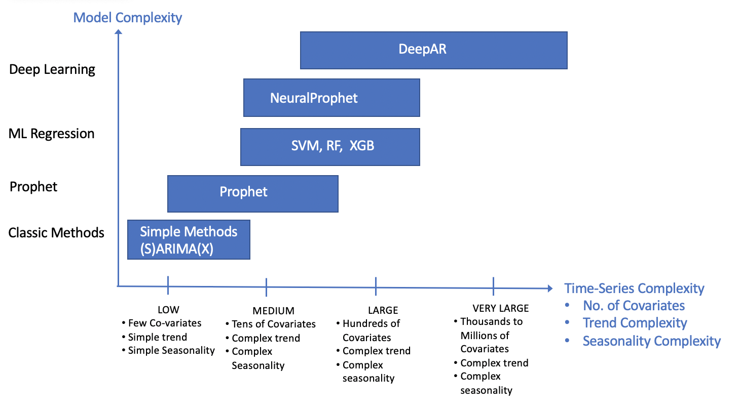
With all these options, businesses are challenged to choose the most effective model and technology for their forecasting applications. For example, countless technical publications argue the merits of one model over another, reporting better performance, such as ARIMA methods over Prophet, DeepAR, and ML algorithms, or visa versa. There is no one best model for all scenarios. For human-in-the-loop analysis, analysts often pick a model based on ease of use and the model’s ability to solve the problem but don’t worry too much about optimizing model efficiency. However, as automation and problem complexity scale, picking an effective and efficient model becomes a key concern. Ultimately, considerations based on the time-series data complexity, computational load, and forecasting accuracy will determine the model selection.
Based on the review of model characteristics, Figure 1 provides simplified guidance for applying the models. For example, for low complexity time-series, a few covariates, simple trend, and seasonality, ARIMA-based models are likely to be the most efficient and provide good accuracy. The Prophet model handles low to medium complexity cases, including tens of covariates, with complex trend and seasonality. For medium to large-scale cases, including tens of covariates, complex trend, and seasonality, ML models such as Random Forest and XGB models can solve the problem. However, they do not explicitly exploit temporal nature. Therefore, to ensure achieving the ultimate predictive performance, they should be compared to deep-learning models or Prophet.
Deep-learning forecasting models offer several advantages. DeepAR, can uniquely handle very-large complexity time-series with multivariate forecasts and is usually the best choice at very-large scale. Training time will be a significant factor for recursive based models (i.e., DeepAR); thus, for medium to large scale problems, NeuralProphet is likely to train faster. Deep-learning models are significantly more complicated to set up and run. Consequently, for medium to large scale problems (up to ~100 covariates), NeuralProphet may provide improved accuracy relative to the predictive analytics models. It is worth emphasizing that there is no one best model for all circumstances. Empirical performance studies will determine the best model.
Summary and Conclusions
Forecasting is an indispensable tool in the business planning process; and a unique problem where optimized solutions exploit the temporal nature of the data. With the acceleration of digital process automation, forecasting models and frameworks present new use cases beyond the small-scale spreadsheet oriented analysis of the past. These realistic use cases are driving new model innovation - they require automation, model usability by non-forecast experts, automation and integration into business processes, and models that scale up to thousands or millions of simultaneous time-series.
Recently, a wave of innovations has significantly improved forecasting models for scale, usability, and accuracy. Modern forecasting models offer a suite of solutions to handle small, medium, large, and very-large-scale forecasting scenarios. Classical models, such as ARIMA, are capable of handling low time-series complexity. For low to medium scale problems, Prophet is a powerful model and offers ease of use by non-forecast experts. Data scientists have frequently employed ML methods, such as SVM (Support Vector Machine), Random Forest (RF), and Extreme Gradient Boosting (XG), for large-scale problems with potentially hundreds of time-series. The deep-learning models offer several advantages relative to the predictive analytics models. NeuralProphet exploits the time characteristics of the problem for medium to large scale problems. DeepAR can handle hundreds to potentially millions of simultaneous time-series. Ultimately the best model for the specific application will result from an empirical evaluation that considers forecasting accuracy and implementation efficiency.
This article provides an overview of the significant advancements in forecasting methods and presents a list of realistic medium to large-scale use cases. A set of tables summarizing forecasting models from small-scale to very-large-scale serves as a cheat sheet for future reference. In consideration of efficiency for scalable processing, guidance for applying forecasting models is provided. In conclusion, this article presents an aligned view across data science, business use-cases, and forecasting for incorporating modern forecasting methods within digital business process automation.
References and Further Reading
[1] Wikipedia. Autoregressive model. https://en.wikipedia.org/wiki/Autoregressive_model.
[2] R. J. Hyndman and G. Athanasopoulos. Forecasting: principles and practice. OTEXTS, 2nd edition. https://otexts.com/fpp2/.
[3] Wikipedia. Exponential Smoothing. https://en.wikipedia.org/wiki/Exponential_smoothing.
[4] B. Letham S.J. Taylor. Prophet, forecasting at Scale. 2017. https://doi.org/10.7287/peerj.preprints.3190v2l.
[5] O. B. Sezer, M. U. Gudelek, A. M. Ozbayoglu, Financial Time Series Forecasting with Deep Learning: A Systematic Literature Review: 2005 - 2019. https://arxiv.org/abs/1911.13288.
[6] David Salinas, Valentin Flunkert, and Jan Gasthaus. Deepar: Probabilistic forecasting with autoregressive recurrent networks. February 2019. https://arxiv.org/pdf/1704.04110.pdf, arXiv 1704.04110.7
[7] Github. Neural Prophet. November 2020. https://github.com/ourownstory/neural_prophet